Build your first model
Start from an empty workbook and build a working staff-cost model — dimensions, series, formulas and your own data — then use it to find something the company's own summary hides.
A company has three years of headcount and salary history and a hiring plan for next year, both split by department. Salaries rise each year by an approved percentage. You have been asked to model the staff budget for 2024 to 2026 and forecast 2027.
You will build it from an empty workbook. Nothing is pre-loaded, and by the end the model will have told you something about the company that its own summary hides. If you would rather see the finished model first — or compare yours against it afterwards — it is published in Demo models as Walkthrough demo.
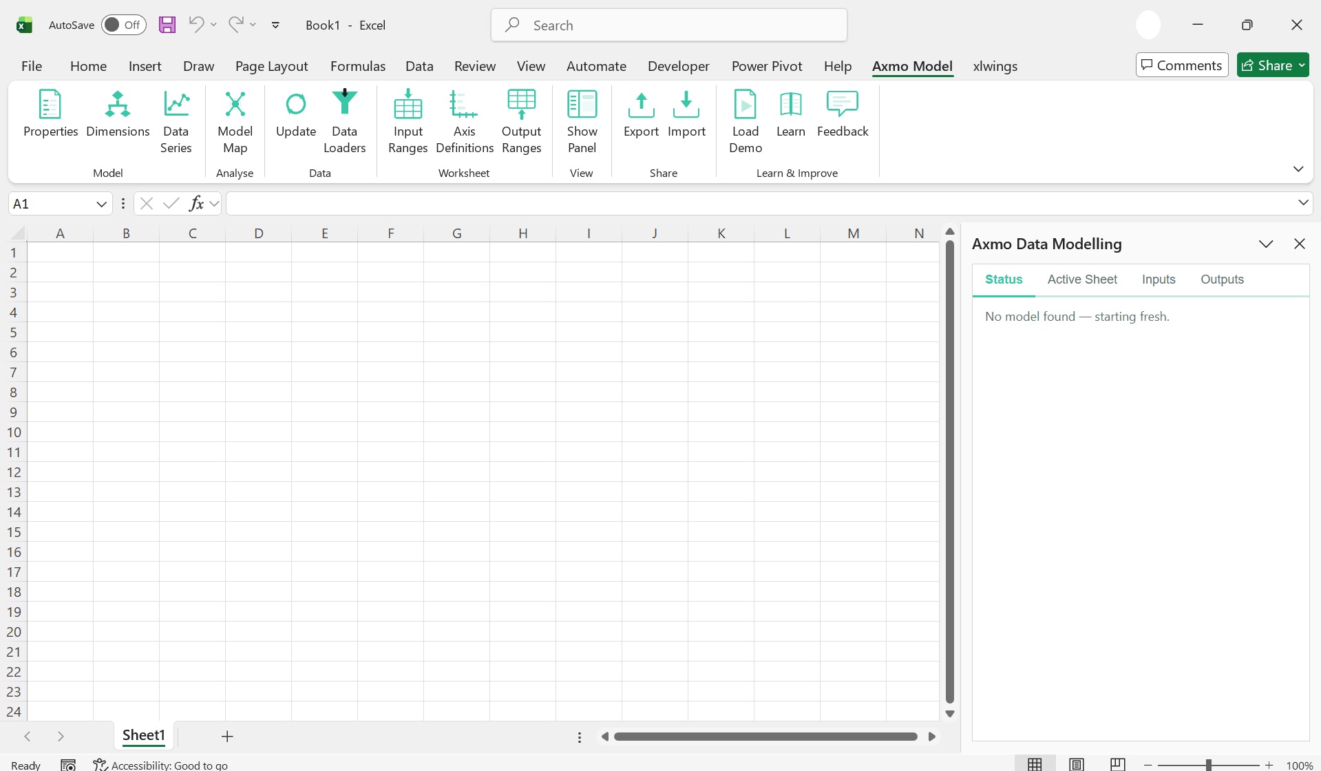
Start a new workbook, click Axmo Model, then Show panel.
Part A — Dimensions
A dimension is an axis your figures vary along. This model has two: who, and when.
Company
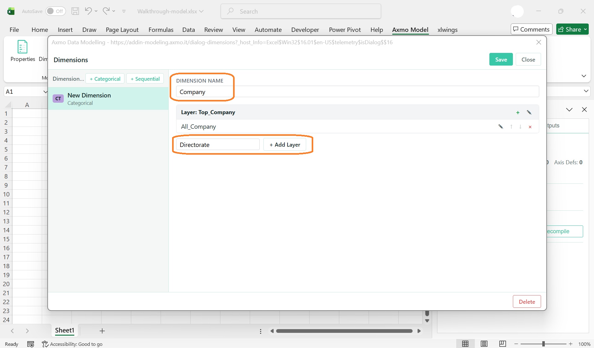
Click + Categorical. Rename it Company — the top layer and its consolidation element follow the name.
Add a layer: type Directorate, then + Add Layer.
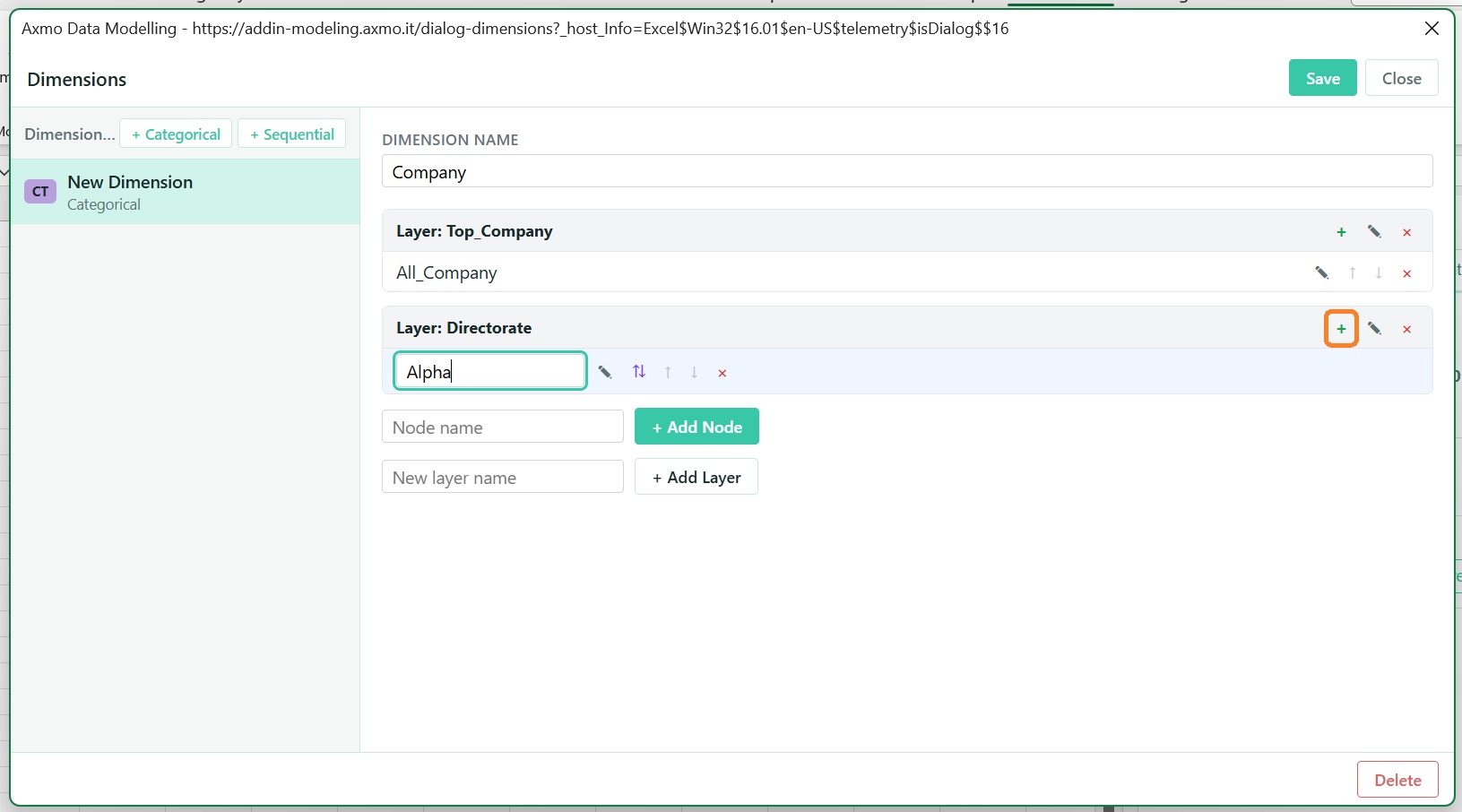
Add its first element with the green + on the layer row: choose the parent, type Alpha, press Enter.
Add Beta the same way.
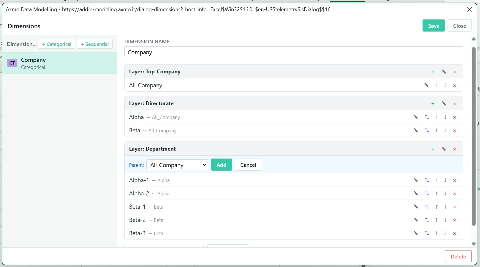
Now a Department layer, and five elements — Alpha-1 and Alpha-2 under Alpha, Beta-1, Beta-2 and
Beta-3 under Beta. Choose the parent each time. The picker offers every element above the layer you
are adding to, not only the layer directly above it, because Axmo lets a child hang from any higher layer.
The buttons to the right of each element rename it, move it, re-parent it or delete it. Save whenever you like. Check the shape against the figure below and Save.
Time
Click + Sequential. Name it Time, kind Time, level Year, start 2024, end defined by end point,
end 2027. Preview — four elements — then Confirm and Save.
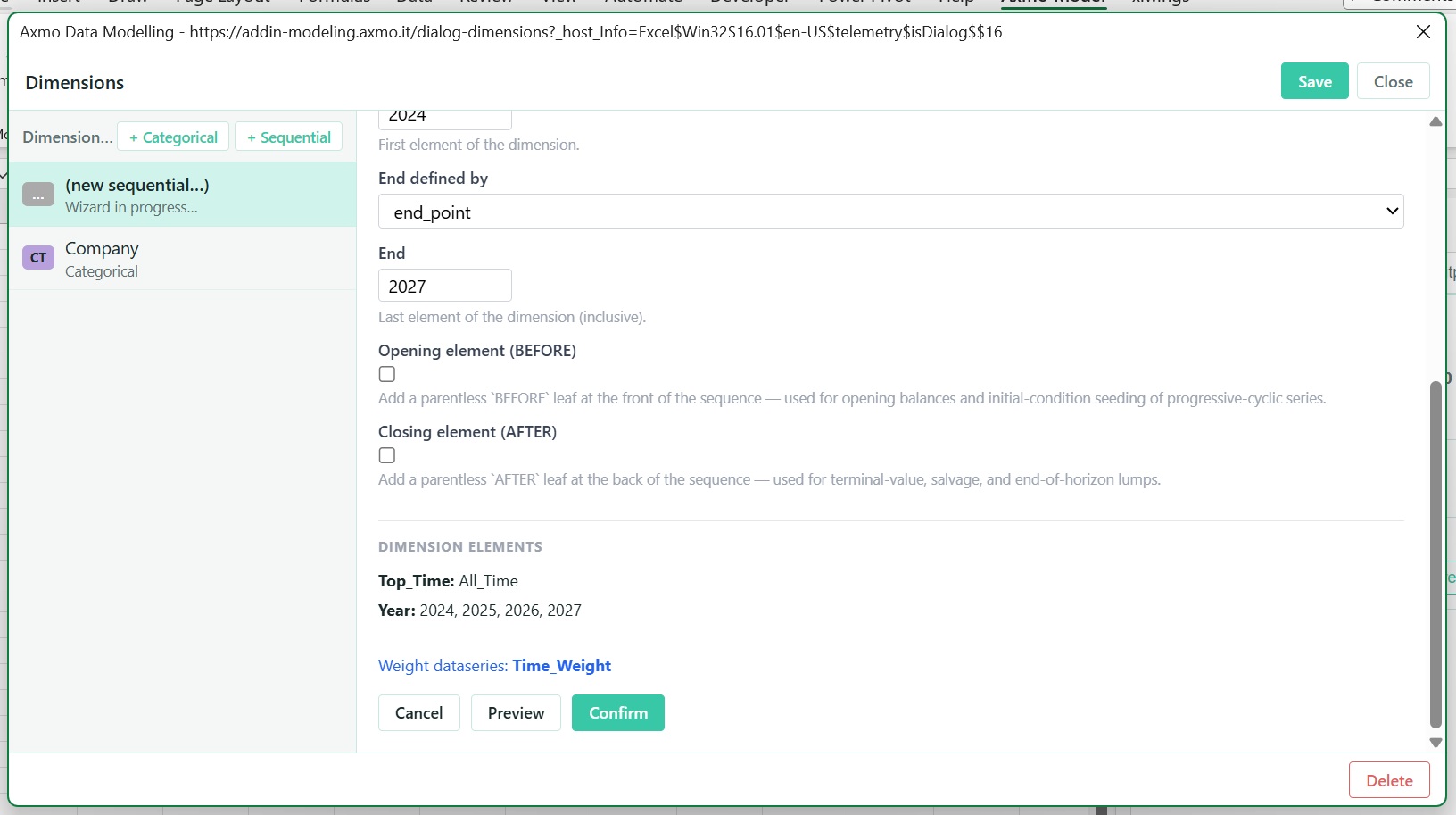
A sequential dimension is generated rather than typed, and its elements have a known order. That order is what
[Year[-1]] will step along in Part B.
Your Data Series list will also show Time_Weight. Axmo creates it automatically whenever a Time dimension
is built — it holds the length of each period in days. You did not add it, and nothing in this model uses it.
Part B — Data series
A data series is a named quantity. Input series hold values you type or load. Calculated series hold a formula, evaluated separately at every coordinate.
The four inputs
Click + Input, name it Joiners Persons, leave both dimensions connected, roll-up SUM, Save.
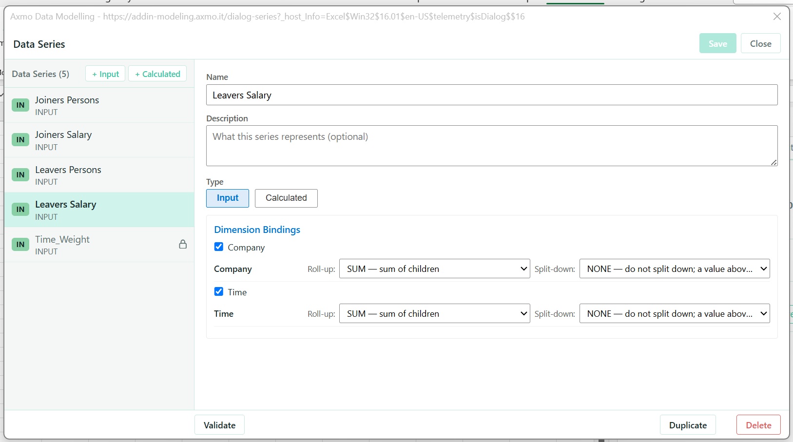
Three more the same way: Leavers Persons, Joiners Salary, Leavers Salary.
Roll-up is chosen per series and per dimension, and it is how the total gets made. SUM is right for people
arriving and money paid out. Nothing about the data tells Axmo that, which is why you say it.
One input that is not per department
Year End Salary Increase, % — untick Company, and set the Time roll-up to NONE.
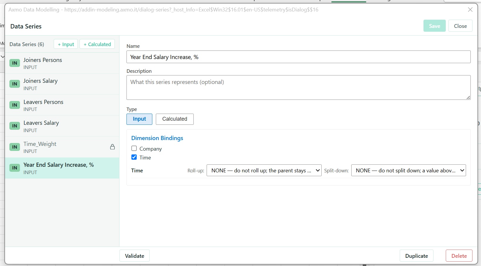
Worth pausing on. The policy is one number a year, the same in every department, so the series has no reason
to vary by Company. Read at any department it gives the same figure. And NONE, because there is no
meaningful total of a percentage across four years.
The calculated series
Click + Calculated, name it Headcount, bindings Company SUM and Time AVG, and the leaf formula:
Nz(Headcount[Year[-1]], 0) + Joiners Persons - Leavers PersonsRead it as a sentence: this year's headcount is last year's, plus joiners, minus leavers. [Year[-1]] steps
back one year. Nz supplies 0 for 2024, where there is no previous year to step to. A series that refers to
its own earlier value is a recurrence, and Axmo works out that it has to be computed year by year.
Time roll-up is AVG here because headcount is a stock. Adding four years of it would count every person four
times.
The rest are the same three steps — name, settings, formula — so only the settings are given:
| Name | Company | Time | Formula |
|---|---|---|---|
Staff Cost | SUM | AVG | Nz(Staff Cost[Year[-1]] * (1 + [Year End Salary Increase, %][Year[-1]]), 0) + Joiners Salary - Leavers Salary |
Average Salary | FORMULA | FORMULA | Staff Cost / Headcount |
Staff Cost Share | FORMULA | FORMULA | Staff Cost / Staff Cost[All_Company] |
Staff Cost Change To Previous Year, % | FORMULA | AVG | IF(Year@ <> 1, (Staff Cost - Staff Cost[Year[-1]]) / Staff Cost[Year[-1]]) |
Average Salary Change To Previous Year, % | FORMULA | AVG | IF(Year@ <> 1, (Average Salary - Average Salary[Year[-1]]) / Average Salary[Year[-1]]) |
Two of these are worth stopping on.
Staff Cost reads the increase at [Year[-1]]. A year-end rise lands on the following year's payroll.
Read it at the current year instead and 2027 would quietly get no rise at all, because the policy table ends
in 2026 — the model would still compute, and the forecast would be wrong.
FORMULA roll-up means the formula runs at the total as well as at the leaves. Average Salary at
Alpha is Alpha's cost divided by Alpha's headcount — not the average of its two departments' averages, which
is a different and meaningless number. A ratio is never summed.
Check your list against the figure below.
![The Data Series dialog headed Total: 12, its list at the top and beginning Average Salary, Average Salary Change To Previ… and Headcount. Staff Cost Change To Previous Year, % is open on the right with Company roll-up FORMULA, Time roll-up AVG, and a formula reading IF(Year@ <> 1, (Staff Cost - Staff Cost[Year[-1]]) / Staff Cost[Year[-1]]).](/_astro/walkthrough-series-list.BEdJiUkA.jpg)
Part C — Connecting to data
Make a new sheet called InputData. Paste the first table into A1 and the second into I1.
One thing to notice in the data. 2024 has joiners in every department and no leavers anywhere, and its
joiner salaries are far larger than any other year's. That is the opening position arriving: the model has
no separate series for the workforce that already existed, so 2024 loads it through Joiners. From 2025 the
columns mean what they say.
| Year | Department | Joiners Persons | Leavers Persons | Joiners Salary | Leavers Salary |
|---|---|---|---|---|---|
| 2024 | Alpha-1 | 20 | 0 | 1000000 | 0 |
| 2024 | Alpha-2 | 15 | 0 | 810000 | 0 |
| 2024 | Beta-1 | 12 | 0 | 720000 | 0 |
| 2024 | Beta-2 | 10 | 0 | 640000 | 0 |
| 2024 | Beta-3 | 8 | 0 | 544000 | 0 |
| 2025 | Alpha-1 | 5 | 2 | 250000 | 104000 |
| 2025 | Alpha-2 | 4 | 2 | 216000 | 112000 |
| 2025 | Beta-1 | 3 | 3 | 225000 | 186000 |
| 2025 | Beta-2 | 2 | 2 | 164000 | 132000 |
| 2025 | Beta-3 | 2 | 2 | 172000 | 140000 |
| 2026 | Alpha-1 | 5 | 2 | 245000 | 106000 |
| 2026 | Alpha-2 | 4 | 2 | 220000 | 114000 |
| 2026 | Beta-1 | 3 | 3 | 240000 | 201000 |
| 2026 | Beta-2 | 2 | 2 | 174000 | 144000 |
| 2026 | Beta-3 | 2 | 2 | 188000 | 154000 |
| 2027 | Alpha-1 | 6 | 2 | 294000 | 108000 |
| 2027 | Alpha-2 | 4 | 2 | 220000 | 118000 |
| 2027 | Beta-1 | 3 | 3 | 258000 | 219000 |
| 2027 | Beta-2 | 2 | 2 | 186000 | 154000 |
| 2027 | Beta-3 | 2 | 2 | 200000 | 168000 |
| Year | YE Salary Increase |
|---|---|
| 2024 | 3% |
| 2025 | 4% |
| 2026 | 5% |
Select the larger table, right-click, and run Create Input Range from the Axmo group at the bottom of the
menu. (The Input Ranges editor does the same thing: + Add, then Use selected.) Name it
Department Year data, Has headers on, Add row number off. Save.
Click + Series Loader. Target series Joiners Persons, value column Joiners Persons, duplicate handling
Block. Then + Add beside Target series three more times, for Leavers Persons, Joiners Salary and
Leavers Salary — the column names match the series names.
Under Dimension mappings, Company comes from the Department column and Time from the Year column.
Save.
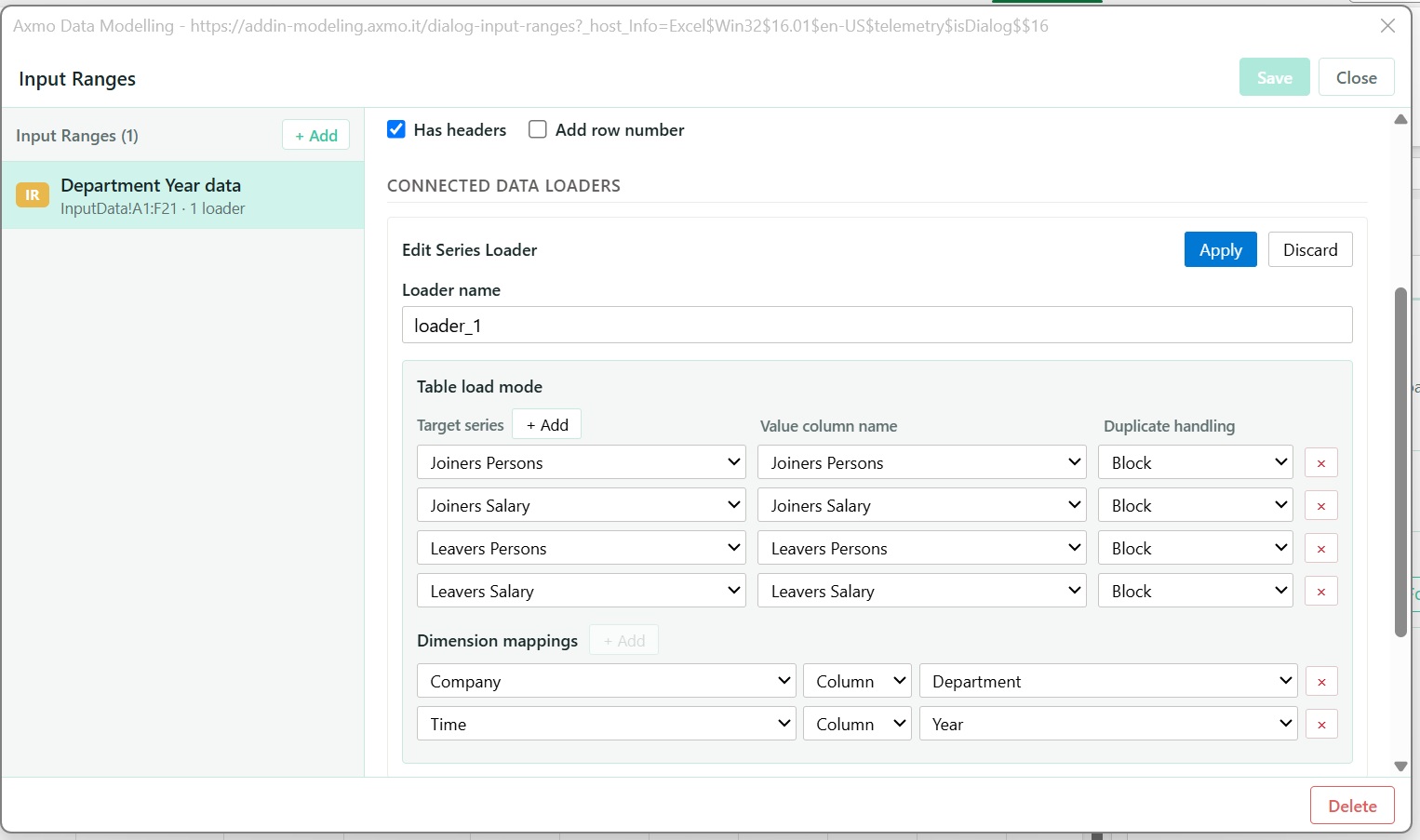
The mapping is how a spreadsheet row becomes a coordinate. Alpha-1 in the Department column is matched to
the element you created in Part A, so the spelling has to agree.
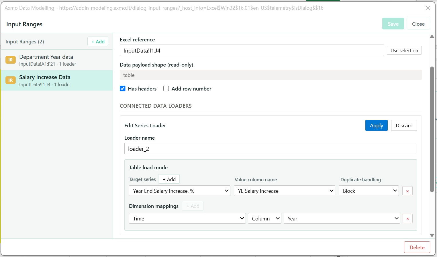
Now the second table, the same way: input range Salary Increase Data, one target
Year End Salary Increase, % from the YE Salary Increase column, duplicate handling Block, Time mapped
to the Year column. Save and close.
Part D — Does it work?
Press Update on the panel. The status becomes Up to date. If something is wrong, the panel tells you what and where — nothing is silently skipped.
In any empty cell with a little room to its right and below:
=DS.DATA("SC_YtY_Change := [Staff Cost Change To Previous Year, %][All_Company]; AS_YtY_Change := [Average Salary Change To Previous Year, %][All_Company]; YE_Increase := [Year End Salary Increase, %][Year[-1]]", "Year", "2024")Format the result as a percentage with one decimal. The third argument drops 2024, which has no previous year to compare against.
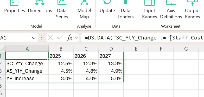
:= become the row labels.| 2025 | 2026 | 2027 | |
|---|---|---|---|
SC_YtY_Change | 12.5% | 12.3% | 13.3% |
AS_YtY_Change | 4.5% | 4.8% | 4.9% |
YE_Increase | 3.0% | 4.0% | 5.0% |
Staff cost is growing at roughly three times the pay policy, while pay per head tracks the policy within a point. So the growth is people, not pay — and at company level the rises look exactly as approved.
That second line is the one worth doubting.
Part E — A report, and what it shows
Building it
Find a free area six columns wide and forty-nine rows deep. Right-click its top-left cell and run Create
Output Range. (Or open the editor and use Use Selection, or type the anchor as Sheet!Cell.)
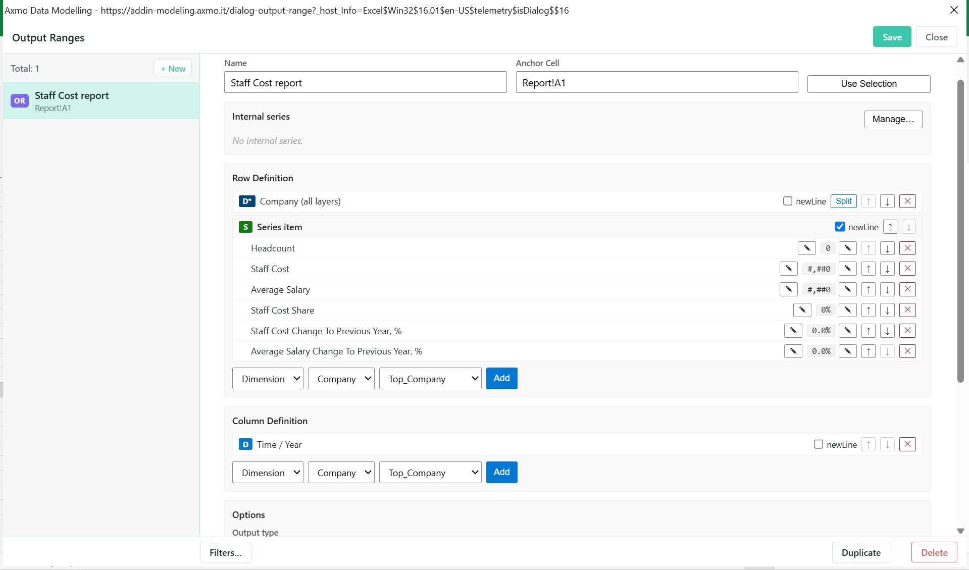
Row definition: Dimension → Company → whole dimension → Add.
Column definition: Dimension → Time → Year → Add.
Then add the series to the row definition. Series → Pick → Headcount → Add, then click the f button
on that row and enter 0 as the format. The others follow: Staff Cost and Average Salary as #,##0,
Staff Cost Share as 0%, and both change series as 0.0%.
Give every series a format. An output cell with no format keeps whatever format was there before it, so a report that grows by a row will show yesterday's percentages under today's headcount.
Check newLine is on for the series row, leave the output type as Report, and make sure Show column headers, Show row labels and Show data are all on. Save, close, and Update.
Reading it
The company view said pay per head is tracking policy. Test it one level down.
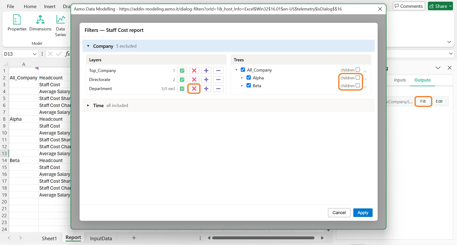
On the panel, open Active Sheet (or Outputs), find Staff Cost report and click Filt. Remove the
Department layer — the red cross on its row, or deselect the children of Alpha and Beta in the Trees
panel — and Apply.
| Average salary, year on year | 2025 | 2026 | 2027 |
|---|---|---|---|
| policy | 3.0% | 4.0% | 5.0% |
| Alpha | 2.2% | 2.7% | 3.1% |
| Beta | 8.4% | 9.0% | 9.6% |
Neither directorate is anywhere near the policy, and their errors nearly cancel. Beta's headcount is 30 in every one of the four years — the directorate that is not growing at all is the one whose pay per head is running at nearly twice the approved rise.
Put the departments back and the same split appears inside each directorate.
Asking a further question without building anything
You can add a calculation to a report without adding a series to the model. In the Output Ranges editor, in the row definition, choose Series → Expression and type:
AS_Joiners := IF(Joiners Persons <> 0, Joiners Salary / Joiners Persons)Add, format #,##0. Then the same for:
AS_Leavers := IF(Leavers Persons <> 0, Leavers Salary / Leavers Persons)Save and Update.
| 2025 | joiners | leavers |
|---|---|---|
| Alpha | 51,778 | 54,000 |
| Beta | 80,143 | 65,429 |
There it is. Alpha replaces the people who leave with people costing slightly less. Beta replaces them at a 22% premium — and by 2027 Alpha is 9% below its leavers while Beta is still 19% above.
Neither directorate is doing anything visible at company level. One is buying growth by hiring below its own average; the other is holding headcount flat while its cost per head climbs. The summary said the pay rises were as approved, and it was right — by coincidence.
One check worth noticing
For Beta and its departments, Staff Cost Change and Average Salary Change are identical. For Alpha they
are far apart. That is not a quirk: where headcount is flat the two must agree, and where it grows the gap
between them is the growth. You could have found Beta's flat headcount from those two rows alone.
Where to go next
The model has room for more: headcount change year on year, staff turnover, cost per joiner. Each is one more calculated series and no new data.